


Abstract
Climate change loss and damage is a critical part of the international climate policy framework, addressing the residual climate impacts that cannot be avoided through mitigation or adaptation, which disproportionately affect vulnerable communities with limited capacity to recover. Major gaps remain in quantifying loss and damage, including developing equitable, operational mechanisms for financing and redress. Here, our contribution is to show how catastrophe models, as commonly used to explore loss and damages in the insurance and reinsurance industries, can be used to calculate loss and damages in a climate policy sense, addressing this urgent quantification gap in international climate policy. We explore the impact of climate change on inland flood risk in three Global South regions (Chikwawa in Malawi, Hanoi in Vietnam, and Cagayan in the Philippines) and three exposure types (residential buildings, agricultural crops, and population) to demonstrate the ability and potential flexibility of catastrophe models to quantify impacts for both economic and non-economic loss and damage. We show that standard catastrophe model metrics can be used to quantify climate policy loss and damage and discuss how they can be used to guide and evaluate adaptation and disaster risk resilience measures. We also show how new metrics can be developed to better suit catastrophe models to this application, including through novel use of a relative wealth metric to explore a social vulnerability dimension. We also discuss and summarise the challenges that remain to be overcome, including sourcing high-quality exposure and vulnerability data and confronting the deeply uncertain climate change information at the scales of interest for climate policy loss and damage. For the latter, we propose a “storylines” framework to tractably sample the uncertainty space. Progress in this area will need meaningful collaboration between stakeholders, developers, local experts, and vulnerable communities, to increase the quality of the data and ensure that the economic and non-economic losses are appropriately, legitimately, and justly chosen and quantified. Our key message is that users and developers of catastrophe models within (re)insurance can leverage their tools and expertise to make much needed and meaningful contributions to the broad issues of climate change loss(es) and damage(s) (e.g., climate finance), but only through extensive collaboration outside of the industry.
Key points:
- Climate change “loss and damage” – the third pillar of international climate policy with adaptation and mitigation – is in urgent need of quantitative tools.
- Standard catastrophe model frameworks used in (re)insurance can fulfil this need and can be adapted to account for many different loss types, including non-economic losses.
- Their use in this manner needs collaboration and engagement with a wide range of stakeholders, including vulnerable communities.
1. Introduction
While the focus of international climate policy has been mitigation (reducing greenhouse gas emissions) and adap- tation (managing the impacts of climate change), loss and damage has become recognised as a third pillar, addressing the residual impacts of climate change that occur when mitigation and adaptation efforts are insufficient or infeasible. Through- out this paper, we use the terms “loss” and “damage” in line with their meaning in international climate policy – broader in scope than definitions common to the insurance industry, as discussed further in this introduction.
Climate change loss and damage was formally recognised by Article 8 of the Paris Agreement, arising from the 2015 United Nations (UN) Framework Convention on Climate Change (UNFCCC) 21st Conference of the Parties (COP21), which stated an ambition of “averting, minimising, and addressing loss and damage associated with the adverse effects of climate change” (UNFCCC, 2016) particularly in vulnerable and developing countries. Seen as an important step towards climate justice, this prompted increased debate and discussion as to the scope and definition of loss and damagea, particularly whether it should also include adaptation measures to climate change (e.g., Boyd et al., 2017; Mechler et al., 2019), as well as how it should embrace economic, non-economic, and indirect losses and damages (Serdeczny, 2019; Richards, 2022). While a lack of standards and frameworks to quantify harm, review evidence of impacts, and inform eligibility for support has meant that efforts to address loss and damage have been slow (e.g., Otto and Fabian, 2024), progress has been made more urgent with the agreement to establish loss and damage financing to support climate-vulnerable countries at COP27 (e.g., McDonnell, 2023 and refs. therein) (with continuing discussions at later COPs).
Here, building on other work (CISL, 2023), we argue that catastrophe (cat) models, as widely used in the insurance industry, can be used to address some core challenges for loss and damage in international climate policy. Broadly speaking, cat models are tools to quantify risk, traditionally being used to ensure the price and capital allocation of insurance and reinsurance is sufficient, with more recent uses in parametric insurance and disaster risk financing (Mitchell-Wallace et al., 2017; World Bank, 2024a). In contrast, much of the climate change literature and international climate policy discourse exploits integrated assessment models (IAMs) to assess economic costs of mitigation options and climate damages (e.g., Weyant, 2017; IPCC, 2022). While these models simulate the relevant interactions of different systems (e.g., economy, energy, land use), they have faced longstanding criticism for their limited spatial and sectoral resolution (e.g., Keppo et al., 2021) as well as more fundamental criticisms on the magnitude of the economic damages that some models project (e.g., Keen et al., 2021). Cat models, on the other hand, provide quantitative information at meaningful spatial scales and, as we demonstrate here, can be structured to consider economic and non-economic losses and damages. Through this paper, we aim to bridge the gap between the financial tools already in use by the insurance industry and the need for quantitative information for international climate policy, chiefly by providing quantitative information at meaningful spatial scales.
We demonstrate the utility of cat models for loss and damage by exploring climate change-driven shifts in flood risk in three distinct Global South case study regions. Floods are among the most destructive natural disasters worldwide, affecting 1.6 billion people and causing USD $651 billion of economic damage between 2000 and 2019 (CRED-UNDRR, 2020). By combining flood models and climate projections, numerous studies have explored changes in future flood risk, which may increase or decrease in different regions, as well as its impacts and potential adaptation strategies (Ward et al., 2017; Dottori et al., 2018, 2023; Willner et al., 2018; Yamamoto et al., 2021; Bates, 2022). While a diverse range of flood adaptation methods exist to reduce losses (Kreibich et al., 2015; Hill et al., 2023), flood protection standards are often lower in more vulnerable regions (Scussolini et al., 2016; Rozenberg and Fay, 2019). Moreover, as 89% of the world’s flood-exposed population live in low and middle-income countries, a focus on exposure of monetary assets – as per a standard cost-benefit analysis – would drive flood protection measures away from these vulnerable regions (Rentschler et al., 2022). Therefore, a broad understanding of future flood risk is vital from a loss and damage perspective, to guide building resilience in vulnerable communities and highlight priority areas where vulnerability can be reduced (McDermott, 2022; Rentschler et al., 2022).
Cat model developers have begun to focus more on flooding resulting from climate change in recent years as global flood risk and losses have increased (e.g., Franco et al., 2020; Bates et al., 2023). Working from a conceptually simple risk framework of hazard, exposure, and vulnerability components, cat models provide an attractive and tractable means to quantify financial losses from flood risk. Key components of flood cat models include a long, high-resolution, synthetic time series of flood event footprints (“event sets”), corresponding flood hazard maps for the events, the ability to quantify flood risk for a portfolio of locations, and the ability to explore different flood-vulnerability relationships. Furthermore, alongside physical data to validate the hazard component, data on insured losses provide a rich source of evaluation material, ensuring models are fit-for-purpose within the insurance industry. At the same time, these simple components can be adjusted, including to account for the impact of climate change and to assess a range of “exposures” and their vulnerability (i.e., not just buildings). This opens the door to using cat models beyond their standard insurance applications.
The standard output metrics of cat models are well-suited to usefully quantify impact for climate change loss and damage. For example, the expected impact (or loss) in a given year from a natural hazard is captured by the average annual loss (AAL), which we focus on in this study. The change in AAL between simulations representative of two different climates (or other chosen metric) is a robust quantitative measure of the change in risk, which could be used in a loss and damage framework. Moreover, high-resolution spatially disaggregated versions of such metrics can not only be used to identify hotspots of risk to climate change, i.e., those with high peril vulnerability, but can also be combined with indicators of social vulnerability. This adds a social dimension to quantitative loss estimates, helping to guide decision making around loss and damage to priority locations, including identifying the adaptation required to combat future risks (Mechler et al., 2019). In this study, we demonstrate this process by first producing high-resolution spatial estimates of flood losses under climate change and integrating our results with high-resolution social vulnerability estimates to identify hotspots of both high flood risk and high social vulnerability, i.e., those areas which have high combined vulnerability derived from both peril and social sources.
Quantifying non-economic loss and damage due to climate change is challenging precisely because they cannot easily be monetised or assigned value through the market (e.g., Barnett et al., 2016; Serdeczny, 2019). Non-economic loss and damage broadly captures impacts on individuals, society, or the environment, and is particularly important in relation to those vulnerable communities at risk of being overlooked in traditional economic risk assessments (Cao et al., 2023). Yet it is seldom considered in planning and policy (Pill, 2022), including for decisions such as prioritising adaptation measures in response to potential future climate change threats (Serdeczny et al., 2016). While cat models are typically used to quantify economic losses to assets (such as buildings) in the (re)insurance industry, we will argue here that their flexible framework allows the exposure of a portfolio of any type of asset to be assessed, provided the relationship between hazard and loss can be quantified.
The aim of this study is to show how cat models can be leveraged to provide a quantitative tool for climate change loss and damage. We demonstrate this through three sub-national flood risk case studies in Global South countries that are also part of the Vulnerable Twenty economies who are “systematically vulnerable to climate change” (https://www.v-20.org): Chikwawa, a highly rural district of Malawi; Hanoi, a province-level municipality in Vietnam consisting of a highly urbanised area with surrounding rural regions; and Cagayan, a province in the Philippines with both rural and urban elements. Using simulations for both a present day and 2°C global warming scenario, we demonstrate the utility of a cat model framework in accommodating various dimensions of loss and damage by quantifying economic losses from residential damage and crop yield reduction, as well as non-economic loss in terms of population affected. To this end, we extend a recent study that used cat models to inform a process for financing (CISL, 2023).
The rest of this study is organised as follows. Section 2 presents more information on the case study regions. Section 3 briefly describes the JBA cat model and its configuration and inputs for this study. Section 4 presents an overview of the results for each case study region, followed by a more detailed spatial analysis of losses at high resolution both directly and in conjunction with high-resolution socioeconomic indicators. Section 5 considers the broader issues and open questions that remain. Finally, Section 6 presents our conclusions.
2. Case study regions
The following sub-sections describe our three case study regions. Maps identifying each case study location within their respective countries are shown in Figure 1.
2.1. Chikwawa District, Malawi
Malawi is classed as one of the world’s 45 Least Developed Countries (LDCs), with around 70% of the population falling below the poverty line and 80% relying on agriculture for their income (World Bank, 2024b). The Shire River valley in southern Malawi has a high risk of flooding due to both its rainfall, characterised by dry and rainy seasons (Jury, 2014), and drainage system, particularly in the south of the country, with an estimated 100,000 people affected every year (World Bank, 2019). At the same time, its citizens’ dependence on agriculture, attachment to the land, and lack of mobility means relocation is rarely an attractive option (Mixed Migration Centre, 2023). Chikwawa is a rural district in southern Malawi. It is among the most exposed and vulnerable regions to flooding in the country (Mwale et al., 2015; Šakić Trogrlić et al., 2018), and was heavily impacted by Tropical Storm Ana in January 2022, which saw 190,000 internally displaced people across southern Malawi (iDMC, 2023).
2.2. Hanoi, Vietnam
Hanoi, both a capital city and province-level municipality, is in the Red River Delta region of northern Vietnam and has a high population density and population of ~8.5 million people as of 2022 (General Statistics Office of Vietnam, 2023). Large parts of the urbanised areas of Hanoi are protected by dikes; however, recent urbanisation and economic development (Luo et al., 2018), a low-lying geography, and the fact that some residential areas remain outside of the dike’s protection, makes it vulnerable to flooding and flood losses (World Bank, 2016; Sai et al., 2020; Anh et al., 2021). Flooding causes considerable impacts each year in Vietnam (Nguyen et al., 2021), including economic loss as well as health and wellbeing impacts (Bich et al., 2011; Hudson et al., 2019).
2.3. Cagayan, the Philippines
Cagayan, a forested province in the north of the Philippines on the island of Luzon, is a major agricultural supplier and has a population of ~1.3 million (Philippine Statistics Authority, 2022). The Philippines is one of the most impacted countries in terms of disaster displacement, exposed to multiple geological and hydrometeorological hazards (iDMC, 2023 and refs. therein). Flooding is frequent and is exacerbated by factors such as deforestation in many locations (Calang, 2017). In 2020, Typhoon Vamco caused widespread flooding across the broader Cagayan Valley region, with especially large impacts in the Cagayan province (OCHA, 2020).
3. Catastrophe model framework and simulations
We use JBA Risk Management’s flood cat model, a proprietary model used extensively in the (re)insurance, financial, development, and disaster risk reduction sectors that is designed to quantify flood risk by integrating hazard, exposure, and vulnerability components. This section briefly summarises the framework and the input datasets we used. The focus is not on the precise details of the model itself but rather the utility of any suitably flexible cat modelling framework to address the challenge of quantifying climate change losses and damages. This also applies to our choice of inputs, such as our vulnerability functions and driving climate model data, where different choices could have been made. We discuss these uncertainties in more detail in section 5.
For further information on the cat model and the underlying flood hazard maps, we invite the reader to consult studies in the literature where the tools and data have been exploited (e.g., Kay et al., 2018; D’Ayla et al., 2020; Becher et al., 2023; Darlington et al., 2024).
3.1. Hazard data
Globally, the hazard component consists of over 15 million plausible fluvial (river) and pluvial (surface water) flood events (the “event set”), which occur with a range of probabilities (return periods) under the climate of interest. The present day (baseline) event set is built with a synthetic precipitation time series (Keef et al., 2013) and rainfall-runoff models (Jakeman et al., 1990; Andrews and Guillaume, 2014), calibrated with historical rainfall (Saha et al., 2010), climate (Kottek et al., 2006), and land cover (Zobler, 1999; Arino et al., 2012) data. Flood depths and extents are determined by reference to JBA’s high-resolution (30 m) global flood hazard maps, incorporating both fluvial and pluvial flooding (Lamb et al., 2009; D’Ayala et al., 2020; Massam et al., 2023).
Events under future climates are generated by scaling the baseline event set with return period change factors, which estimate the magnitude and spatial pattern of the climate change signal. The return period change factors map the intensity of a future event to a baseline equivalent in return period space (e.g., a change factor of 2 means that a future 100-year event has the same intensity as a present-day 200-year event), which enables the model to use return period hazard maps for the present day. Note, the change factor at a given location is fixed for all return periods, which means that, among other things, the change in event intensity is monotonic across return periods.
The change factors themselves are determined using output from global climate models (GCMs). In our case, we used output from one of the UK Met Office GCMs (UKESM1-0-LL) (Sellar et al., 2019) that contributed to the sixth Coupled Model Intercomparison Project (CMIP6) (Eyring et al., 2016), generating an event set for a 2°C global warming scenario (2°C above pre-industrial temperatures), a level of warming that is broadly consistent with mid-century projections for a range of GCMs and scenarios (IPCC, 2021). In brief, the change factors are calculated by generating a “climate uplift” (which can be negative) to the present day median annual maximum rainfall or river flow, which is then re-ranked in a series of ~30 years of present day data to give the change factor via the inverse Gingorten formula (Gringorten, 1963). While the change factor approach is simplified, this methodological choice respects the large uncertainty in GCM output and in determining spatially resolved future climate projections (e.g., Shepherd, 2014).
3.2. Vulnerability functions
The vulnerability component quantifies the expected impact for a given hazard intensity (i.e., the peril component of vulnerability) using depth-damage curves, which are critical for quantifying loss (Kreibich et al., 2009; Merz et al., 2013; Lazzarin et al., 2022). In this study, we are concerned with agricultural crops and residential buildings. We also calculate a population-weighted impact using the portfolio of exposures, which is explained in the following section below.
We use flood depth-damage curves from the Joint Research Commission (JRC) (Huizinga et al., 2017). These are derived primarily from data in the literature, covering multiple continents and exposure types as well as providing continent-level normalised damage functions and country-level maximum damage values, which we use to translate the curves into quantitative losses. We linearly interpolated the curves to give damage estimates at flood depth intervals of 0.1m, which increases the sensitivity of loss estimation to flooding and more closely imitates the continuous functions often used to quantify flood damages (e.g., Merz and Thieken, 2009).
The JRC depth-damage curves have known limitations. For instance, residential damage is treated uniformly, with no distinction between building types, and agricultural damage is provided only at the country level in euros per hectare, with no information on crop type. These constraints stem from limited data availability which we discuss further in Section 5.
3.3. Exposure data
Locations of exposed assets were compiled from various open data sources, allowing us to demonstrate the flexibility of cat models for different exposure types. Details of the data sources, justification for their use, and any modification are provided below. Analysis was carried out at the resolution of the exposure for each exposure type. Maps showing the final exposure datasets are shown in Figure 1. While we can expect exposures – and their vulnerabilities – to evolve through time, we kept this aspect constant in all our simulations, which simplifies the analysis and isolates the hazard component of any future change in risk.
Population: Population data were sourced from WorldPop (Tatem, 2017) and consist of population counts for 2020 at 100 m resolution. In our analysis, population estimates are disaggregated to individual exposures based on spatially gridded population density data available from WorldPop. Individual exposure locations are assessed independently against the flood hazard maps. We define the “exposed population” as that encountering flooding of any depth. The “AAL” for this exposure represents the average number of people affected per year per grid point, referred to as AALpop hereafter.
Agricultural Crops: Agricultural crop exposure data were sourced from the Global Land Analysis & Discovery Lab Global Land Cover and Land Use Change dataset (Potapov et al., 2022), extracting the 30 metre pixels classified as cropland for 2020. The value of exposed crop at each point was calculated following Huizinga et al. (2017), estimating the value added by 30 m2 of cropland for each country in 2020 by dividing the gross domestic product contributed through agriculture in each country (FAO agriculture, forestry, and fishing data via FAOSTAT; https://www.fao.org/faostat/en/) by the total agricultural area in each country (World Bank data; https://data.worldbank.org). The AAL for this exposure represents the average value lost per year per grid point, referred to as AALcrop hereafter.
Residential Buildings: Residential building exposure data were sourced from the Global Human Settlement Layer (Pesaresi and Politis, 2023). Data representing residential buildings was extracted and the resolution was resampled from 10 metre to 30 metre to reduce the computational burden. The value exposed at each grid point was taken from the Joint Research Commission estimates for land-use based maximum damages for residential buildings (Huizinga et al., 2017), adjusted to the exposure data’s resolution. The AAL for this exposure represents the average value damaged per year per grid point, referred to as AALres hereafter.
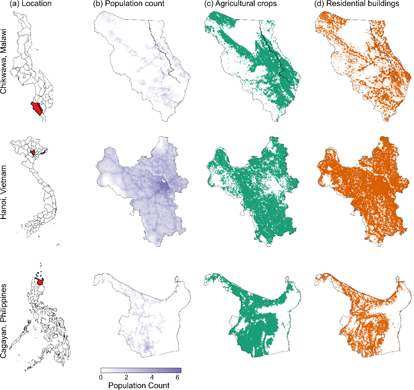
Figure 1: Case study regions and the distribution of exposure types, showing (a) the location of each sub-national region within the larger country and the exposure locations for (b) population count (additionally coloured by density), (c) grids classified as agricultural crops in the Global Land Analysis & Discovery Lab Global Land Cover and Land Use Change dataset (Potapov et al., 2022), and (d) the location of and residential buildings according to the Global Human Settlement Layer dataset (Pesaresi and Politis, 2023).
3.4. Socioeconomic vulnerability data
To meet our aim of demonstrating how cat model outputs can provide a social vulnerability dimension, we also use the relative wealth index (RWI) (Chi et al., 2022). This is constructed by estimating the spatial distribution of wealth for all low- and middle-income countries at a resolution of 2.4 km using machine learning methods, providing a dataset that can be suitably combined with the high-resolution cat model output. We note that wealth alone is just one proxy for socioeconomic vulnerability and more complex, multi-indicator versions have been created (e.g., Edmonds et al., 2020), which would be a natural extension to this work.
4. Results
The analysis presented below demonstrates a quantification of the impact of climate change on flood risk for our three case study regions and three exposure types. However, the “demonstration” aspect is important: we are not seeking to generate precise values (which, not least, would require a deeper exploration of uncertainty and better on-the-ground information concerning vulnerability) but instead show the utility of cat models in generating the quantities and insights that would be useful for climate change losses and damages. Moreover, as noted above, our simulations only explore the impact of hazard change rather than exposure and social vulnerability. To this end, we do not present monetary values in this analysis, expressing losses as relative changes. We return to these broader points concerning limitations, uncertainties, and development needs in Section 5.
4.1. Total expected annual loss
The overall change in AAL between the present day (hereafter “baseline”) and 2°C warming scenario provides an indication of risk to climate change-related flood losses for each exposure type considered (Table 1). In our demonstration, Hanoi exhibits the highest risk overall when using change in AAL as the indicator of risk, showing the greatest percentage increases in AAL. For all exposure types in Hanoi, increases in AAL under the 2°C warming scenario exceed 60% compared to baseline, exceeding 70% for residential buildings (AALres). Cagayan also shows increases in losses under the 2°C warming scenario, although at close to 35% across all exposure types, the relative change is approximately 1/2 to 2/3 that for Hanoi. Chikwawa has the lowest overall risk of increasing flood damage, with negligible changes in AAL for all exposure types (1% decrease to ~2% increase).
| Exposure Type | % Change | ||
|---|---|---|---|
| Chikwawa | Hanoi | Cagayan | |
| Population (AALpop) | –0.6 | 63.2 | 37.6 |
| Agriculture (AALcrop) | –0.7 | 68.9 | 37.5 |
| Residential Buildings (AALres) | 1.8 | 71.3 | 34.2 |
4.2. Spatial distribution of losses
To demonstrate the ability of cat models to estimate losses at high spatial resolutions whilst maintaining realistic results, we consider the spatial distribution of the AAL and its change between baseline and the 2°C warming scenario within each region, aggregating the metric to 0.01° resolution, which is ~1 km at the equator. We present our analysis by region in sub-sections below.
Throughout this section, we report losses using a ‘relative AAL’ metric (Figures 3–5, panels (a) and (b)). For population, the relative AALpop is calculated using the average annual number of people exposed to flooding as a percentage of the total population count for each grid point; for residential buildings and agricultural crops, the relative AALres and AALcrop, respectively, are calculated using the average annual economic loss as a percentage of the total value exposed at each grid point.
Particularly for the latter two exposure types, reporting the results in this way avoids placing unnecessary emphasis on the value of assets, which is important given the assumptions involved in their calculation, and brings focus to the general trends both spatially and between scenarios. The openly available vulnerability functions allow for consistency between countries; however, the assumptions made during their calculation (Huizinga et al., 2017) also means the outputs presented here are more suited to estimating general trends across regions and through time. The change in the relative AAL is used to quantify the impact of climate change (Figures 3–5, panel (c)).
To introduce a socioeconomic vulnerability dimension, our analysis also includes an RWI-weighting of the relative AAL. This provides an insight into the relationship between flood risk and relative social vulnerability across the case study regions, which, for example, can emphasise areas where high flood risk and high vulnerability coincide. RWI values for each region are converted to deciles to help capture the variability in RWI across each region more clearly (i.e., put into 10 equally distributed groups and given a value of 1 (low) to 10 (high)). The choice to calculate deciles of RWI reflects the fact that the RWI is not comparable between regions, meaning it is important to avoid methods which encourage direct comparison between RWI values. Deciles of the RWI values in the original RWI dataset are shown in Figure 2.
The RWI deciles are assigned to the aggregated cat model output using a nearest neighbour approach. RWI-weighted results are only shown for points where the distance between the exposure point and the RWI data point is less than twice the resolution of the RWI data (4.8 km). This means that we do not assume distant locations have similar vulnerabilities. The weighted AAL is calculated by dividing the relative AAL by the RWI decile. This means that, compared to the unweighted relative AALs, expected losses in areas with the highest RWIs (indicating highest wealth) are down-weighted the most, whereas expected losses in areas with the lowest RWIs (indicating lowest wealth) expected losses remain more similar (Figures 3–5, panel (d)). The locations with high weighted relative AAL values therefore represent high flood risk coinciding with high socioeconomic vulnerability.
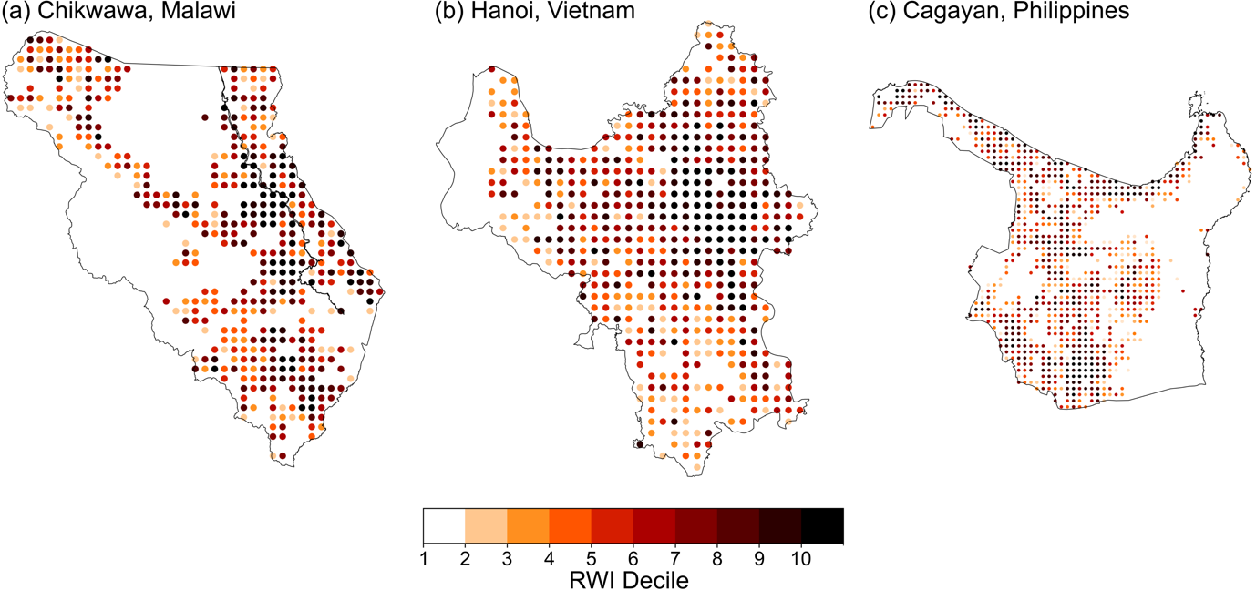
Figure 2: Maps showing the deciles of the RWI data points calculated for each case study region on the original RWI dataset for (a) Chikwawa, (b) Hanoi, and (c) Cagayan.
4.2.1. Chikwawa, Malawi
For baseline, flood risk impacts ~14% of the population, ~14% of agricultural crop value, and ~8% of residential building value when aggregating the relative AALs across the whole region. The change in relative AALs between the baseline and the 2°C warming scenario is generally negligible, with a few points of increasing AAL mainly seen for population affected (AALpop). This latter result reflects the assumption that population is considered ‘affected’ by any flood depth exceeding a threshold of 0.2 m, meaning that this exposure type is more sensitive compared to the others. An area of decreasing relative AALs surrounding the river is seen in the northeast of the region, consistent across the exposure types (Figure 3c), suggesting decreased risk to flooding in this area under the 2°C warming scenario. However, there is large uncertainty as to the magnitude and direction of precipitation change under global warming over Malawi (Warnatzsch and Reay, 2019).
The RWI-weighted relative AALs in Chikwawa reveal a patchy pattern of flood risk and social vulnerability co-location, with a particularly dense area of high RWI-weighted AALs in the southeast of the district, suggesting this is an area of high relative combined vulnerability within Chikwawa province, as well as high flood risk under the 2°C warming scenario (Figure 3d). These patterns are consistent with areas of higher and lower vulnerability in a previous assessment of flood vulnerability (Mwale et al., 2015). That assessment pointed to its use of coarse spatial resolution data as a limitation in identifying some of the finer-scale patterns in vulnerability. With our higher-resolution approach, we can see both the general patterns of large areas of higher and lower vulnerability, alongside the finer details within these areas where the AAL and RWI-weighted relative AAL change significantly over short distances (Figure 3d). However, establishing the veracity of our results would require further validation.
4.2.2. Hanoi, Vietnam
For Hanoi, flood risk impacts ~9% for population in the baseline, which more than doubles to ~20% in the 2°C warming scenario when aggregating relative AALs across the whole region. For agricultural crops, the aggregate relative AALcrop increases from ~7% in baseline to ~11% in the 2°C warming scenario, with a similar increase in AALres from ~7% to ~12% for residential buildings. The spatial distribution of changes in relative AALs between baseline and climate change scenarios shows a mix of areas of negligible changes and areas of positive changes, with no locations showing decreasing flood risk (Figure 4c). Areas of particularly high increases in relative AALs are seen in the northeast and southwest edges of the province, away from the highly urbanised central region, coinciding more with rural areas. These also coincide with some of the greatest RWI-weighted AALs, with the highest of these clustered towards the southwest edge of the region (Figure 4d). This suggests that, for Hanoi, the highest RWI-weighted AALs are driven both by high flood risk and high socioeconomic vulnerability.
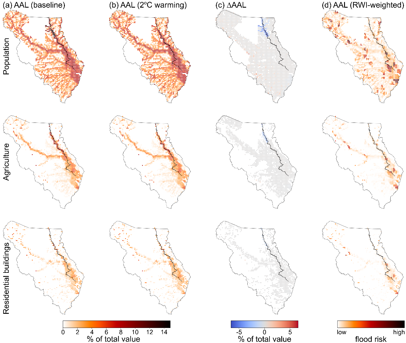
Figure 3: Cat model results for Chikwawa showing “AAL” for the different exposure types as a percentage of the total exposed value at each grid point, aggregated to 0.01° for (a) the baseline scenario, (b) the 2°C warming scenario, (c) the change in relative AAL between these, and (d) the 2°C warming AAL weighted by the relative wealth index (RWI) to indicate the combined peril and socioeconomic vulnerability. Results are shown for (top) population, (middle) agricultural crops, and (bottom) residential buildings. In all panels, areas shown in white indicate either no exposure or a relative AAL of zero.
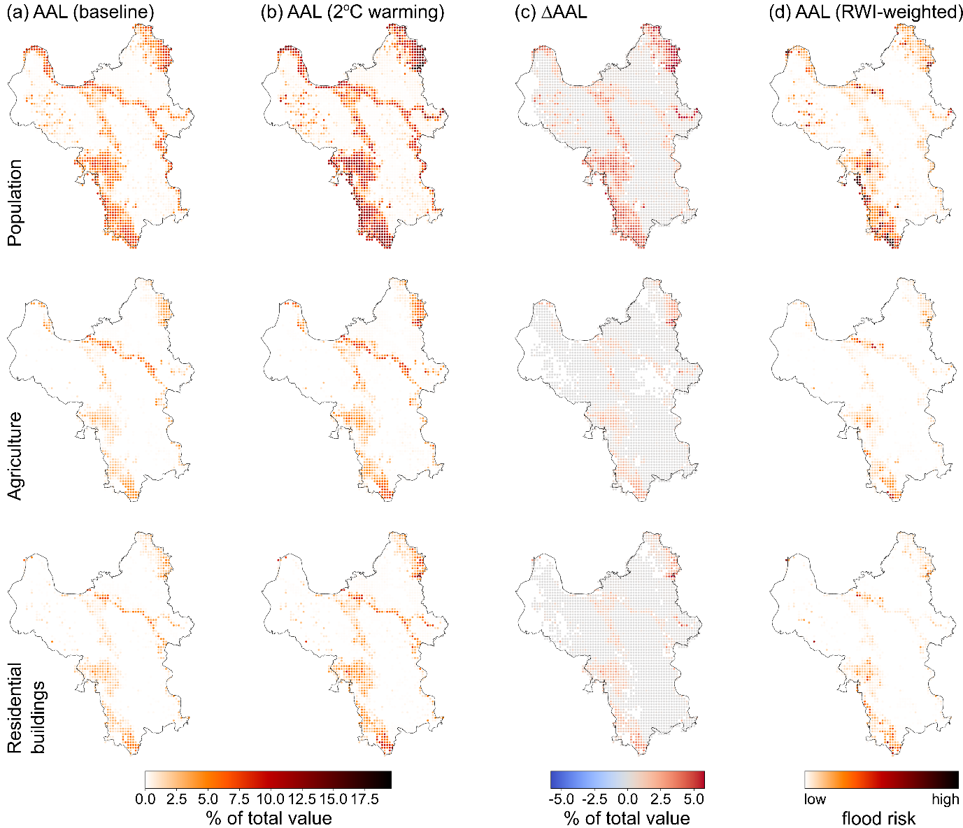
Figure 4: Cat model results for Hanoi showing “AAL” for the different exposure types as a percentage of the total exposed value at each grid point, aggregated to 0.01° for (a) the baseline scenario, (b) 2°C warming scenario, (c) the change in relative AAL between these, and (d) the 2°C warming AAL weighted by the RWI to indicate the combined peril and socioeconomic vulnerability. Results are shown for (top) population, (middle) agricultural crops, and (bottom) residential buildings. In all panels, areas shown in white indicate either no exposure or a relative AAL of zero.
4.2.3. Cagayan, Philippines
Model results for Cagayan show similar magnitudes of increases in relative AALs to Hanoi. For the baseline, ~9% of the population is affected by flooding in any one year, increasing to ~19% in the 2°C warming scenario, when aggregating relative AALs across the whole region. For agricultural crops, the aggregate loss increases from ~8% of the overall value in baseline to ~12% under the 2°C warming scenario, with a similar increase of ~7% to ~12% for residential buildings (Figures 5a and 5b). In terms of spatial distribution, the changes in relative AAL are dominated by hotspots of positive changes in the northeast and southwest, in among large areas of low or zero changes, and a few locations with small decreases (Figure 5c). Whilst some of the locations of large AAL increases coincide with the largest RWI-weighted AALs, areas of high RWI-weighted risk are seen across the province and are less confined to areas of high flood risk (Figure 5d). This suggests that for some locations in Cagayan, the RWI-weighted AAL is more strongly driven by high socioeconomic vulnerability than high flood risk.
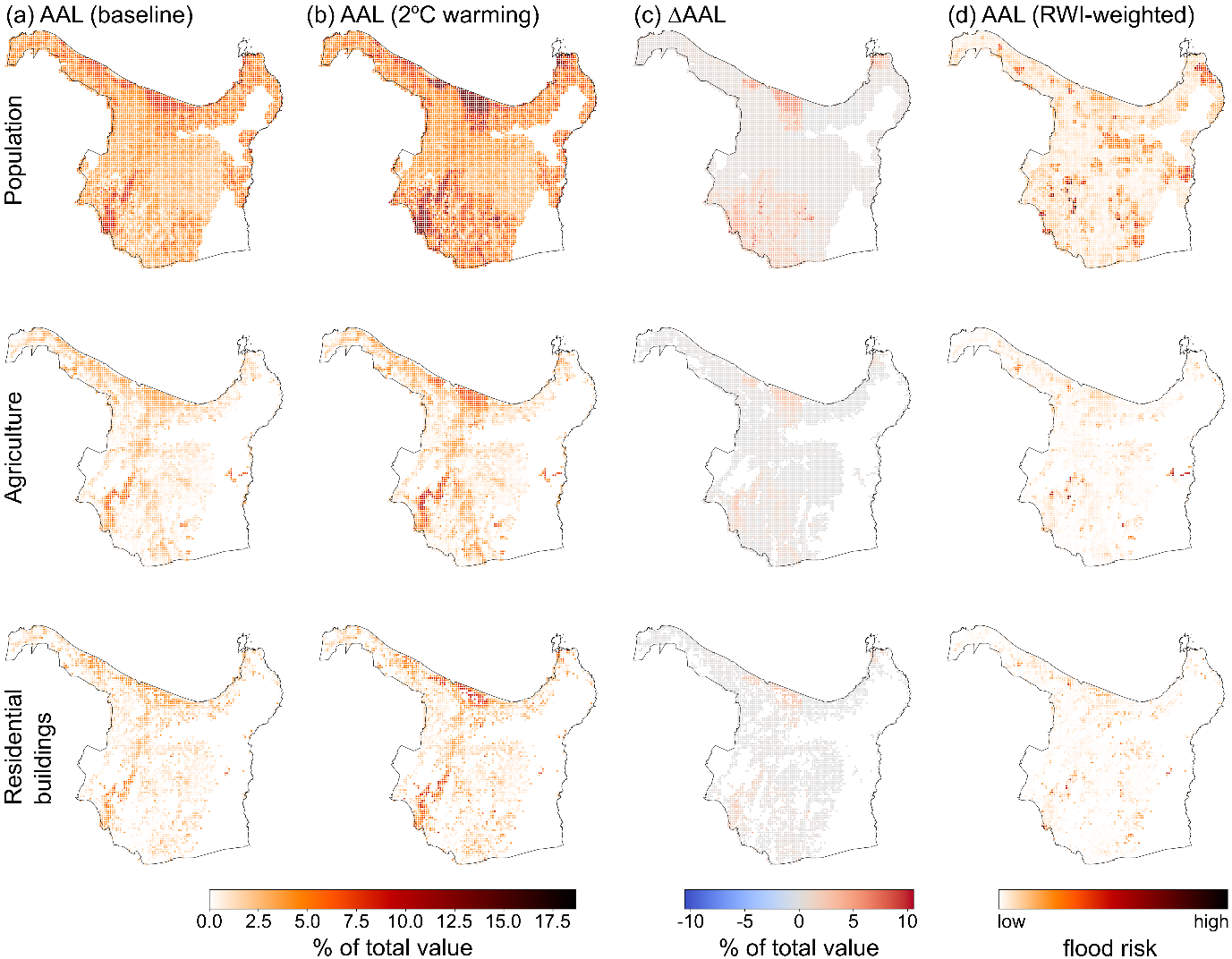
Figure 5: Cat model results for Cagayan showing “AAL” for the different exposure types as a percentage of the total exposed value at each grid point, aggregated to 0.01° for (a) the baseline scenario, (b) the 2°C warming scenario (b), (c) the change in relative AAL between these, and (d) the 2°C warming AAL weighted by the RWI to indicate the combined peril and socioeconomic vulnerability. Results are shown for (top) population, (middle) agricultural crops, and (bottom) residential buildings. Areas shown in white represent either no exposure or a relative AAL of zero.
5. Cat models as tools for loss and damage: reflections and open questions
With the example of flood risk in three Global South countries, we have demonstrated the utility of a cat model framework, augmented with high-resolution geospatial datasets, to quantify loss and damage under climate change. We used a metric based on the average annual loss (AAL), a standard (re)insurance metric, to quantify flood risk under present-day (baseline) conditions and a 2°C warming scenario. Overall, with these simulations, we found that our three chosen regions would face different degrees of change in flood risk under this measure: a ~70% increase for Hanoi, Vietnam; a 35% increase for Cagayan, the Philippines; and a negligible change for Chikwawa, Malawi. These changes hold true for the three exposure types that we investigated: population, residential buildings, and agricultural crops. With the diverse regions and exposure types, our study has provided a glimpse of the flexibility – and underexplored potential – of cat models in a loss and damage framework, which can provide the customisable and context-specific quantitative estimates central to the loss and damage financing process in international climate policy (Otto and Fabian, 2024).
The change in AAL represents the probability-weighted impact of climate change on flood risk and is one candidate metric that could be used to quantify loss(es) and damage(s). By integrating over all possible hazard intensities in the cat model event set, this metric has advantages over comparing the impacts of different scenarios and time periods in integrated assessment models, since the latter will not capture such a broad range of possibilities of hazard events. Similar advantages are also present in other cat model metrics, which may be selected as a stronger evidence base to inform a particular action. For example, one could focus on the change in loss from an event of a given return period, seek to determine a “probable maximum loss”, or explore whether impact is coming from changes in frequent, low-impact events vs infrequent, high-impact events.
Moreover, mediated by their high resolution, flood cat models can help stakeholders target vulnerable localities with practical adaptation measures. For example, in Hanoi province, our results suggest that the largely agricultural south-west of Hanoi province faces the highest flood risk, both under baseline conditions and a 2˚C warming scenario. Flooding has a significant impact on agricultural productivity in Hanoi, leading to compounding impacts such as risk to food supplies (Ha, 2024). Therefore, a spatial analysis of flood risk is crucial for effectively directing loss and damage finance, ensuring resources are allocated to the most vulnerable regions to mitigate future impacts. This is a key advantage of a cat model-based framework to quantify climate change loss and damages over the more widely used integrated assessment models.
While offering advantages over direct use of climate model outputs, cat models are still dependent on the output of climate models to project the change in hazard. Such projections are fraught with deep uncertainties at the spatial scales of interest, with different climate models often projecting opposite signs of change in variables like precipitation (Seneviratne et al., 2021). As well as model deficiencies (e.g., Wehner et al., 2021), this pertains to uncertainties in how large-scale weather patterns might be altered under climate change, in turn driven by the highly uncertain response of atmospheric dynamics to greenhouse gas forcing (e.g., Shepherd, 2014). In practice, this means that any use of a cat model framework to quantify losses and damages should go beyond our demonstration and explore a range of possibilities for how climate change could impact natural hazards in the region(s) of interest, such as by using a storylines framework (Shepherd et al., 2018).
In a storylines framework, cat models could be used to explore a range of plausible regional climate changes and the required adaptation measures to mitigate any increase in loss and damage that would otherwise result. This could include integrating data on flood defences and other mitigation strategies, including projections of urbanisation and population changes, and quantifying the cost of inaction (it is generally understood that the cost of disaster risk reduction measures is less than the cost of recovery (Mechler, 2016). Indeed, the JBA cat model has already been used to explore these kinds of questions recently (Sarailidis et al., 2023).
At the same time, we must recognise that uncertainty extends beyond the hazard component of the cat model to include the exposure and social vulnerability components necessary for investigating storylines of adaptation. In conducting this study, a lack of data meant pragmatic choices had to be made concerning exposures and their vulnerabilities, including a uniform distribution of value across exposure points and the use of generalised vulnerability functions to translate flood depth into damage, whereas we would expect both to be spatially heterogeneous. Moreover, sourcing information of sufficient quality at a regional level was a key challenge in this study and generating exposure portfolios from available, high-resolution data sources introduces uncertainty arising from data accuracy. Recognising, quantifying, and reducing these and other uncertainties is needed, working across academia, industry, and with local actors (Balzter et al., 2023; Déroche, 2023). Given the complexities and non-linearities that are pervasive in cat models, the importance of the different uncertainty sources on the final output uncertainty is generally not immediately obvious (Sarailidis, 2023). Strategies such as global sensitivity analysis can help identify the dominant drivers of uncertainty and help developers focus efforts for model improvement (Sarrazin et al., 2016).
Beyond the technical considerations for designing and implementing simulations, engagement in the loss and damage space requires cat model developers and users to engage with fields, concepts, and collaborators beyond the domains usually explored in (re)insurance. With many seemingly well-established concepts occupying a highly contested space – poverty metrics (e.g., Alkire and Santos, 2014; Ravallion, 2020), climate adaptation governance (e.g., Persson, 2019), climate resilience (e.g., Mikulewicz, 2019), human rights (McNamara et al., 2023) to name but a few – one might question the tractability of the endeavour. Ways forward include recognising that a perfect technical solution will not emerge without challenges and that approaches need to be transdisciplinary, enveloping a range of skills and perspectives and being codesigned and coproduced with stakeholders (e.g., Balzter et al., 2023). This is particularly relevant for non-economic losses, which are not always quantifiable in a traditional economic sense (Tschakert et al., 2019). For instance, one might begin (as we did) by quantifying the affected population: although a residence may not be damaged, damage to surrounding businesses, infrastructure, food production or cultural sites and sacred places could indirectly “damage” wellbeing or livelihood (e.g., Walker-Springett et al., 2017; Steadman et al., 2022). However, making legitimate assessments and quantifications needs representatives of the region(s) under question: “nothing about us without us”.
In addition to ethical considerations, these questions have a political dimension too, as they are likely to have a profound impact on how a loss and damage fund will be operationalised. For instance, given the prevailing economic paradigm that focuses on quantifiable losses, it is not only crucial to include non-economic losses into loss and damage models and finance but also include vulnerable communities into the very process of assessing and valuing those losses (McShane, 2017). This would be a more just approach while also going some way to closing the “adaptation gap” (UNEP, 2023) and to better direct the loss and damage finance that currently does not reach the most vulnerable communities (IFRC, 2022; Oxfam, 2023; Wilkinson et al., 2023).
In summary, bridging the gap between the insurance industry and international climate policy community requires convening expertise from across sectors: financial institutions, government agencies, frontline organisations, and communities directly exposed to climate risk. Each sector contributes essential knowledge: insurers bring tools to quantify and price risk; local institutions and community groups offer context-specific insight and access; and policymakers create the frameworks through which action is channelled. Together, they can adapt catastrophe models for purposes beyond indemnity payouts, refining them into tools for assessing climate-related loss and damage. Coupled with high-resolution hazard data and socioeconomic scenarios and storylines, these models can address forward-looking questions about how risk will change. Anticipating such shifts is vital for designing effective strategies and reducing the loss and damages from future extremes.
6. Summary and conclusions
In this study, we have demonstrated how catastrophe (cat) models, as commonly used in the insurance and reinsurance industries, can be used to quantify climate change loss(es) and damage(s), fulfilling a key need to make urgent progress in this arena of international climate policy. With a focus on the impact of climate change on inland flood risk in three Global South regions – Chikwawa in Malawi, Hanoi in Vietnam, and Cagayan in the Philippines – and three exposure types – residential buildings, agricultural crops, and population – we have shown the ability and potential flexibility of cat models to quantify impacts for economic and non-economic loss and damage. Their utility is chiefly in their ready-made risk framework, which incorporates hazard, exposure, and vulnerability and generates a range of metrics to explore the impacts of extreme events. Unlike direct use of climate model output, cat models create a multi-thousand-year representation of the climate of interest, meaning that their metrics can reflect the weighted impact of a spectrum of extreme events or focus in on different ends of the extreme event distributions. The change in these metrics between simulations of different climates can be used to quantify loss and damage, as well as guide and evaluate adaptation and disaster risk resilience measures.
Nevertheless, one must consider the quality of the hazard, exposure, and vulnerability data used in the model framework. Here, while we were able to demonstrate the utility of a cat model framework for a range of exposure types, sourcing high-quality exposure and vulnerability data was challenging (the Global South is less well served with this information (e.g., Glas et al., 2019), resulting in the need to make assumptions and pragmatic choices. Moreover, climate change information is deeply uncertain at the scales of interest for loss and damage (Shepherd, 2014). Recognising this, we proposed using a storylines framework (Shepherd et al., 2018) to tractably sample the uncertainty space for future projections, as well as global sensitivity analysis to better understand and quantify inherent cat model uncertainties (Sarrazin et al., 2016).
Finally, and most importantly, building on this proof-of-concept will need meaningful collaboration between stakeholders, developers, local experts and vulnerable communities, to increase the quality of the data and ensure that the economic and non-economic losses are appropriately, legitimately, and justly chosen and quantified (Balzter et al., 2023). It remains essential for the insurance industry to collaborate across sectors – and include the communities directly exposed to climate risk – to extend the use of cat models beyond their traditional insurance applications.
Overall, we hope that demonstrating the application of cat models in the loss and damage domain and highlighting the key challenges encourages future activity, improvements, and collaboration in this crucial space.
Footnotes
- We follow the IPCC Special Report on 1.5°C (IPCC, 2018) and use “loss(es) and damage(s)” (lower case) to refer broadly to the harm from climate change, as opposed to “Loss and Damage” (capital letters), which refers to the wider political debate under the UNFCCC.
References
P.J., 2016. FLOPROS: an evolving global database of flood protection standards. Natural Hazards and Earth System Sciences, 16: 1049–1061. https://doi.org/10.5194/nhess-16-1049-2016
Declarations
Handling Editor: Ioana Dima-West, PhD, Head of Science and Natural Perils, AXA XL
The Journal of Catastrophe Risk and Resilience would like to thank Ioana Dima-West for her role as Handling Editor throughout the peer-review process for this article. We would also like to extend our thanks to the chosen academic reviewers for sharing their expertise and time while undertaking the peer review of this article.
Received: December 18th 2024
Accepted: June 8th 2025
Published: July 2nd 2025
Acknowledgements
The authors are grateful for, and acknowledge the contributions and support of multiple JBA employees, past and present, towards building the models and datasets that were used in this study. Since the UKESM1-0-LL data used in this study was downloaded from the CMIP6 archive, the authors also acknowledge the World Climate Research Programme, which, through its Working Group on Coupled Modelling, coordinated and promoted CMIP6. The authors also thank the climate modelling groups for producing and making available their model output, the Earth System Grid Federation (ESGF) for archiving the data and providing access, and the multiple funding agencies who support CMIP6 and ESGF.
Code and data availability
Those interested in licensing the catastrophe model used in this study should contact hello@jbarisk.com. Details on the other datasets (exposures, vulnerabilities etc.) are available from the citations provided.
Rights and Permissions
Access: This article is Diamond Open Access.
Licencing: Attribution 4.0 International (CC BY 4.0)
DOI: 10.63024/0y4e-cdqp
Article Number: 03.03
ISSN: 3049-7604
Copyright: Copyright remains with the author, and not with the Journal of Catastrophe Risk and Resilience.
Article Citation Details
Galloway, E., et al., 2025. Catastrophe risk models as quantitative tools for climate change loss and damage: A demonstration for flood in Malawi, Vietnam, and the Philippines, Journal of Catastrophe Risk and Resilience, (2025). https://doi.org/10.63024/0y4e-cdqp
Share this article: https://journalofcrr.com/research/03-03-galloway-et-al/